Assessing Pass/Fail Testing When There Are No Failures to Assess
June 1, 1997
In the course of their work, persons involved in manufacturing medical devices are often required to sample and test products or product components. Often this testing involves the collection of what are known as variable data. Variable data are continuous, quantitative data regarding such things as temperature, pressure, and efficiency. By their nature, these types of data provide an enviable precision in measurement, which in turn provides product developers the luxury of small sample sizes without a concomitant loss of statistical power. With such precise data the risk of making a wrong decision concerning products being tested is minimized.
However, quite often product development personnel are called on to sample and test a product, or product component, in which the only information gathered is whether it meets one of two possible outcomes, such as passing or failing a test. This category of information is known as attribute data. Attribute data are a discontinuous form of data resulting in the assignment of discrete values, such as yes or no, go or no-go, 0 or 1, or pass or fail.
Attribute data are often collected by engineers, product designers, product/project managers, and others who require initial basic information about a material or product component in order to judge its suitability for use in a medical device. The usefulness of attribute data in pass/fail testing lies in its allowing user-defined failure criteria to be easily incorporated into research tests or product development laboratory tests--tests whose results, as a rule, are easy to observe and record. In general, if one observes that the test product meets defined criteria, the observation is recorded as a "pass"; if it does not, the observation is recorded as a "fail." The number of passes and fails are then added up, descriptive statistics presented, conclusions drawn, and manufacturing decisions made.
A FALSE SENSE OF SECURITY
However, the results of such attribute tests can be misleading because the risk associated with decision making on the basis of them is often understated, or misunderstood. This is particularly true when samples are tested and no failure events are observed. When failure is observed in a product being tested the logical course of action is to proceed with caution in drawing conclusions about the acceptability of the test product. In other words, there is a recognition of risk brought about by the observation of one or more failures. Conversely, a zero failure rate observed during testing generally leads to a decision to proceed with the product being investigated.
However, there is a risk in drawing conclusions about a product when no testing failures are observed. Zero failure brings about a sense of security that is often false. There is a tendency to forget that even if 10 components were tested without failure, we still can't be absolutely sure how the 11th would have performed. The resulting overoptimism could result in the inclusion of a component in a product, or the introduction of a product into the marketplace, that fails to perform as expected.
A false sense of security is a particular danger when the investigator has not thought about the relationship between risk and sample size. As an example, more risk is involved in stating that a product is acceptable if we sample 10 with no failure from a population than if we sample 500 with no failure from the same population. This is because we derive more information about the population from testing a sample of 500 than from testing a sample of 10. It is more important to know that zero failure occurs in a sample size n than simply that zero failure occurs.
When no failures are found after a particular round of pass/fail testing, the estimated failure rate is zero--if that single test is looked at in isolation. What is often misunderstood in pass/fail testing is that a zero failure rate for the given sample tested does not ensure that the failure rate for the entire product or component population is zero. When no failures are reported during sample testing, the natural tendency is for researchers to overlook the maximum failure rate that could occur for the population as a whole. The maximum failure rate for the population, not the sample, must be understood, and should be part of the risk assessment involved in decision making.
SAMPLE SIZE
What is an appropriate sample size for pass/fail testing? It depends on how critical the product or component being tested is, and how much risk the investigator (scientist, engineer, project manager, decision maker) is willing to accept when deciding whether or not to accept that product or component for manufacture or distribution.
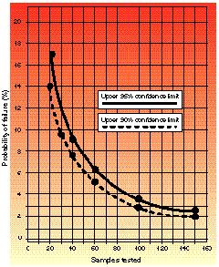
 Figure 1. Upper probability of failure when zero failures are observed, based on 90 and 95% confidence intervals (
 /2). (
 /2 is the risk associated with rejecting the null hypothesis. Its division by 2 addresses the fact that any established rejection region exists in both tails, or ends, of the distribution, and that the probability of error is divided equally between the two tails.)
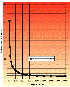
For any given sample size, with zero failures observed, there is an ascribed confidence interval--worked out and tabulated by statisticians--in which the true failure rate will be found.1 Shown in graph form in Figures 1 and 2 are the upper bounds for that failure rate, based upon 90 and 95% confidence intervals ( /2). The advantage to presenting this information in graphic form is that a knowledge of statistical theory is not required to interpret it.
 Figure 2. Upper probability of failure when zero failures are observed.
Figure 1 shows the upper limits at 90 and 95% confidence intervals for failure rate when zero failures are observed. It is clear from the graph that the fact that no failures are observed does not mean that no failures are to be expected in the total population of parts or components; rather, failure may be expected to be as great as that defined by the curves. The graph can be interpreted in several ways by considering the following scenarios.
Example 1. You have just completed a test in which 40 samples were evaluated and you observed 0 failures. From Figure 1, the upper bound for the true failure rate is 8.8%. One can then state that, with 95% confidence, the true failure rate will be contained in an interval not to exceed 8.8% failure.
Example 2. You are required to make a decision about continuing with the development of a product line. Because of time and cost limitations, the decision involves considerable risk. You decide to proceed with development if pass/fail testing indicates a 90% chance that the true failure interval does not exceed a 3% failure rate. How many samples are needed with 0 failures observed? The answer is 100, found by following the 90% confidence limit curve downward until it crosses the 3% probability line. The point of intersection corresponds to 100 on the sample axis.
Example 3. A sample size of 150 is tested with 0 failures observed. From the graph you find that there is a 95% chance that true failure will occur within an interval bounded by an upper limit of 2.4% failure. The question you must ask yourself is this: Am I willing to proceed knowing that I have a 95% chance of product failure that could be as great as 2.4%? In other words, does this risk analysis represent sufficient information about the product under development?
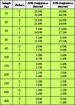
 Table I. Upper boundary of expected failure from 90 and 95% confidence intervals in which true failure probability is expected to be exhibited. The probability of the upper boundary is equal to
  /2.
/2.
The colors of the graphs range from red (danger) to yellow (proceed with caution). If you are pass/fail sampling and observe zero failures from a sample of size n during the test, you should determine where on the confidence limit curves your upper range of failure exists. To do this, locate on the x-axis the number of samples you have tested, then move vertically until you cross either the 90 or 95% confidence curve. The color area you are in will give you a subjective determination of the risk of failure if you proceed with the development of this product (with red equaling higher risk and yellow equaling caution, or lower risk). You may then locate along the y-axis the upper probability of failure occurring when all that you know about this product is that zero failures occurred in your sample size. Notice that the graphs do not contain the color green (go). This is because there is always risk involved.
For further reference, Table I presents the upper limits of expected failure when zero or one occurrence of failure is observed during testing.
CONCLUSION
Statistical analysis shows that in both attributes and variables testing, as the amount of valid information increases, the associated risk in making a decision based on that information decreases. In pass/fail testing this means that the ability to estimate with confidence the upper bounds of the true failure rate when the observed failure rate is zero is critically dependent upon sample size. Thus, decision making is also critically dependent on sample size.
REFERENCES
1. Collet D, Modeling Binary Data, New York, Chapman & Hall, 1991.
2. Fisher RA, and Yates F, Statistical Tables for Biological, Agricultural, and Medical Research, 6th ed, Edinburgh, Oliver and Boyd, 1963.
Thom R. Nichols is senior research statistician and Sheldon Dummer is senior quality engineer at Hollister, Inc. (Libertyville, IL).
Copyright ©1997 Medical Device & Diagnostic Industry
You May Also Like

.png?width=300&auto=webp&quality=80&disable=upscale)
