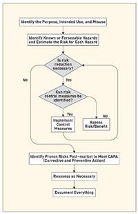
Risk management is defined as the systematic application of policies, procedures, and practices to the tasks of analyzing, evaluating, and controlling risk. In general it involves a three-step procedure for identifying and assessing risks to determine the appropriate measures to be undertaken in case of unacceptable risk levels. ISO 14971 is a worldwide risk management standard for medical device manufacturers.¹ It details the basic steps of the risk analysis process as illustrated in Figure 1. The purpose of this process is to ultimately support reasonably safe products with a systematic, specific, and rational effort.

Risk estimation is commonly made possible through the use of an indicator known as the risk score. The risk score is the combination of the probability of the occurrence of a harm or hazard and the severity of that harm or hazard if it were to occur. To be more precise, probability is the likelihood that the harm or hazard will actually manifest itself, whereas severity is the degree of harm that will result if said event occurs. This broad definition gives rise to several important questions, as follows:

•How can harm and hazard both be used in risk analysis?

•What definition of probability does the risk score really involve?

•What kind of probability-severity combinations can be used for the evaluation of the risk index?

•What are the limits of the widely-used qualitative risk analysis, and are these limitations resolved by the use of a quantitative approach?

•Are current quantitative methods definitive for comparing overall risks?

When attempting to answer these questions, device OEMs may find that the current methods for quantitative and qualitative risk analysis do not accommodate the actual needs for practical use. This article discusses these methods and attempts to explain why medical device manufacturers may be placing too much value on such analysis.

Hazard and Harm: Any Difference?

ISO 14971 defines hazard as the potential source of harm, and the term harm is used to designate the physical injury or damage to the health of people or to property. More simply, hazard is the cause and harm is the end result. Hazards are sometimes used as shorthand for harm in order to focus attention on causation. Such careless terminology, however, can result in observers losing the significance of the effect.

Similarly, harm is sometimes used in risk analysis to retain attention on the ultimate effect, but then causation might get lost. In addition, hazards that occur may be detectable before they cause harm, whereas ultimate harms may not be detectable until after they occur. To illustrate the differences in meaning, three medical-related examples of hazards and harm are listed in Table I.

Furthermore, the cause-effect relationship between hazard and harm may not be direct. Indeed, the path from hazard to harm can be very complex, as shown in the example of a use error–related alarm failure (see Figure 2). This example shows that while a use error associated with having the alarm volume too low may initiate a failure to hear the alarm, there are various intervening design and detection flaws that occur before the initial error results in the death of the patient.

Sources of hazards can be divided into four major categories, as follows:

•Sources inherent to the technology, such as x-rays, electricity, and sharp-edged scalpels.

•Sources related to the design, which may involve internal, technical, or software issues, as well as user interface and human factors concerns.

•Sources associated with manufacturing, such as failure to meet or adequately define the required specifications.

•Sources related to the instructions for use, including that they may be inadequate, incomplete, or confusing.

Probability of Occurrence:What Definition?

To avoid misestimating the likelihood of a harm occurring, risk analysts should properly define the probability used for evaluating the risk index. As suggested in Appendix D of ISO 14971, the definition of probability is highly dependent on the medical device in question. Additionally, defining probabilities as per unit time of use brings forth the concept of the frequency of the occurrence of the harm. The definition, therefore includes the important notion of time in the risk analysis process.

Another important consideration is whether to use absolute measures of probability or to define conditional probabilities based on some relative weight. In other words, should one be concerned with the conditional probability of a certain failure mode occurring given that failure occurs instead of simply considering the absolute probability of a certain failure mode occurring?

Probability and Severity: What Combination?

Risk analysis typically uses a two-dimensional risk chart. Figure 3 provides a visual representation of the probability of harm occurrence on the x-axis and the severity of the harm on the y-axis. Various regions of this two-dimensional space can be defined, such as a generally acceptable (GA) region for which both severity and probability are low, a generally unacceptable (GU) region for which both severity and probability are high. There is also an in-between region sometimes referred to as ALARP (as low as reasonably practicable). Alternately, the two-dimensional space may be simply divided into acceptable and unacceptable risk.¹ The configuration does not account for other important factors such as hazard detectability (which is commonly used in manufacturing risk analysis), hazard correctability, and utility or importance of the device.

Even with the simple division into acceptable and unacceptable, distinction should be made between a premitigation and postmitigation analysis. A risk should generally not be deemed acceptable if it is not reasonably feasible to mitigate it.

The very definition of acceptable and unacceptable in defining zones on the chart is often less than rigorous, and there is no uniformly accepted definition. For example, the typical chart in Figure 3 suggests that a low probability and a high severity combine into a relatively safe region. However, this statement does not apply to reality, as exemplified by after-the-fact analysis of Guidant's defibrillators.^2,3

In spite of their relatively high reliability (i.e., low probability of harm), these devices were considered in an independent report to be unsafe because their use could lead to death (i.e., high severity). Furthermore, the risk could be mitigated, especially with respect to devices as yet unsold. This suggests that high severity is unacceptable even at low probability, especially if the hazard can be reasonably eliminated or controlled. Therefore, the generally unacceptable region should be extended in such cases to cover even low probability levels as shown in Figure 4.

In general, the definition of the risk zones is left to the subjectivity and rational thinking of the risk analyst. Moreover, the chart can be divided into even more zones with defined action plans for each (see Figure 5). Another challenge is locating a possible failure mode on each of the probability and severity scales. Dividing the scales into discrete levels can be helpful. Typically, there are 3–5 division levels on each of the two scales, with the number of divisions being either equal or unequal. Divisions of as many as 10 segments can also be found, although the level of precision implied by such a high number is probably hard to justify.

Table II shows a typical five-level scaling with two alternative probability verbal scales. Figure 6 shows a risk diagram using 5 × 5 scaling with three zones defined. Note that this risk chart has the combination of a high severity and a low probability as acceptable. For the purpose of discussion of such a chart, a matrix notation should be used (assigning a number for each severity and probability level). Note that these numbers have no inherent meaning other than being a marker for the associated division.

In Figure 6, probability and severity scales are denoted by the linear numerical values 1, 2, 3, 4, 5. As a result, a 2-3 designation indicates the region associated with a probability of three and a severity of four. While this matrix notation may help in describing the location of one's estimate, it does not allow for risk comparisons. In particular, all points in the ALARP region may not be equally risky. Between 2-3 and 3-2, which is the more risky? How much improvement is implied in moving from 2-3 to 2-2? In addition, how certain or uncertain is the selection of the discreet value? Because a qualitative approach (i.e. using descriptive terms) does not offer a systematic tool to assess and compare risk, risk analysts often turn towards a quantitative method (i.e. assigning or computing numerical as described below).

Quantification of Risk: Any Improvement?

In order to quantify risk, numerical values can be assigned to each of the positions on the severity and probability scales. This is at first similar to the matrix notation used above, but here the numbers are assumed to be mathematical quantities that can be manipulated mathematically. In particular, these values can be combined by some mathematical formula to compute a number, which is referred to as the risk score (defined earlier) or risk index (RI). First consider an equal and linear numerical scaling which ranges from 1 to 5 for each axis as shown in Table III. To combine the probability (p) and severity (s), a first (and common) approach consists of multiplying the values: RS = p x s.

The results of such a risk score computation are shown in Figure 7. However, this linear multiplication configuration with equal linear scales suffers from five major limitations.

Arbitrariness of Scales. The scale values for probability and severity are essentially arbitrary. There is no reason why the two scales should be the same or different. Similarly, there is no reason why they should be linear or nonlinear. Even linear scales do not divide the space linearly. For example in Table II the highest probability rating is >50%. Therefore, whatever number is assigned to this division still represents only half of the outcomes.

Characterizing the Zones. Linear quantification of estimated risk does not produce any real improvement in zone characterization. Zones must still be subjectively defined, although now with some mathematical restraints.

False Symmetry. The configuration of Figure 7 suffers from a false symmetry, whereby equal values do not necessarily refer to equally risky situations. For example, the value 10 appears twice, but are these equal risks?

False Relativity. It may be tempting to use linear quantification for risk comparison based on the obtained numerical values of the risk index. However, it is irrational to consider a risk score of 16 four times as bad as a risk score of 4. Does improving the system from a risk index of 16 to 4 imply that the risk has been divided by four?

Uncertainty. If there is any uncertainty concerning the probability or severity scale values, it is important to consider how that combined uncertainty can be illustrated in the box configuration of Figure 7. Determining the uncertainty of the risk index is highly dependant on the nature of the combination, be it multiplication or any other mathematical formula.

Such limitations suggest that the linear and equal configuration fails to address the fundamental problems of quantitative risk analysis, and thus, it does not offer any actual improvements compared with the qualitative approach. However, its numerical nature might falsely imply that it is fundamentally meaningful and that the values obtained have inherent meaning.

For comparison, Figure 8 shows the risk scores obtained for the multiplicative rule when unequal and non-linear numerical values are assigned to both the probability and severity axes. In this case, the severity scale is 1, 2, 4, 8, 16 and the probability scale is 1, 3, 5, 7, 9. Note that this scaling is severity biased. This new configuration eliminates false symmetry and also results in higher risk scores at unacceptable regions. The magnification of the risk scores associated with unsafe regions may look more helpful in delimiting the risk zones. However, the risk values still lack a substantial basis. A risk reduction from “56” to “6” does not necessarily indicate a risk reduction of 89%, nor does it result in a more acceptable risk than the one obtained after a one-fourth reduction from “16” to “4” as discussed earlier.

Multiplication is not the only option for combining severity and probability. At least one manufacturer uses the following power law rule calculation: RS = Severity^Probabilty

The results of this calculation for equal 1–5 scales are shown in Figure 9. These values show some false symmetry. There is also an interesting effect for the lowest severity value of 1, since the risk scores remain equal to one even for high probability of harm occurrence. Thus, an important value judgment is built into both the scales and the math. The high-risk score values in the unacceptable regions are interesting in that they are also a direct result of the power law calculation. However, these high numbers do not provide an actual representation of the relative degree of risk, nor do they provide any additional help concerning zone delimitation. The risk index magnification could present a psychological trick in that the unacceptable risks might seem more acceptable. However, it is equally true that improvements resulting in lower scores may seem even more impressive.

Risk Comparisons

Despite the limitations in the numerical meaning of risk scores, it is tempting to seek to combine risks to calculate an overall risk score. To illustrate such a calculation, three hypothetical design alternatives are considered in Table IV. Each project consists of several individual risks for which the probabilities and severities have been qualitatively determined according to the verbal scale of Table IV. Alternative A has five identified risks, alternative B has three, and alternative C has 20, although all of the C risks are relatively modest. Because only one alternative can be chosen for implementation, it is desirable to compare their overall risks.

To attempt this comparison, the probability and severity verbal scales can be replaced by their corresponding numerical values and then multiplication can be used to calculate the risk index for each risk. This is shown in Figures 7 and 8 for two different numerical scales. The final step consists of adding the individual risk indexes to compute the overall risk for each project. There is at best a marginal theoretical basis for adding risk scores, but at least it requires that the individual risks must be mutually exclusive, as will be assumed here. The results for the linear and nonlinear configurations are shown in Tables V and VI respectively.

For the two scaling patterns, the following can be noted:

•Linear Configuration. Project B was found to be the least risky, while Project C presented the highest overall risk, although the absolute difference is small.

•Nonlinear Configuration. Using the nonlinear scales Project C was found to be the least risky, while Project B presented the highest overall risk. However this conclusion is highly dependent on the set of values used for each of the severity and probability scales. The result here is particularly due to the fact that low scores are relatively undervalued, while middle risk scores are assigned heavier weights.

The results of using the two scales' pairs clearly lack consistency. This suggests that relying on the mathematical significance of the assigned numerical value, multiplication, and then addition may lead to bad decision making and thus put patient safety in jeopardy. More basically, it illustrates the fundamental weakness of such risk calculations.

Conclusion

The theoretical soundness of the current quantitative methods used for risk assessment of medical devices is fundamentally weak. Yet many medical device companies rely on such false numerification (i.e., the process of making numerical, and seemingly precise, that which is essentially qualitative) and believe in the significance of the values obtained. However, since these numbers lack a sound basis, it would be generally unwise to deal with these values as if they were actual entities representing some measurable quantity.

The critical weaknesses are that the numerical scaling does not represent tangible or actual data, and the subsequent mathematical calculations are equally suspect. Overvaluing the significance of this numerification can directly affect decision making pertaining to the design or manufacturing of the medical device, especially if one option must be chosen among various alternatives based on a risk minimization criterion. Fortunately, the ultimate conclusion is not that such techniques should be abandoned, but that they must be used with caution and with an understanding of their limitations.

References

1.ISO 14971. 2000(E) “Medical Devices—Application of Risk Management to Medical Devices, Revised.” (Geneva, International Organization for Standardization; 2007).

2.J Fielder, “Moral Blindness and the Guidant Recall,” IEEE Engineering in Medicine and Biology 25, no. 1 (2006): 98–99.

3.R Steinbrook, “The Controversy Over Guidant's Implantable Defibrillators” New England Journal of Medicine, 353, no. 3 (2005): 221–224.

Copyright ©2009 Medical Device & Diagnostic Industry